1D grids

This vignette shows how to obtain a boxplot or histogram given a dataframe of points in a plane.

library(rgrids)
library(ggplot2)

Boxplot

A density analysis in one dimension can be performed on points lying on a line suitably divided into segments, that is, different $x$ and $y = 0$, or on a set of points in the plane which is divided into strips.

If we consider a plane divided into strips, the grouping of points can be shown in a boxplot.
Let’s see how to proceed.

Define dataframe of points

First we define a dataframe of random points

set.seed(1)
    
df_points <- data.frame(x = c(rnorm(n = 5000, mean = -4), 
                              rnorm(n = 5000, mean = 4)), 
                        y = c(rnorm(n = 5000, mean = 1), 
                              rnorm(n = 5000, mean = -1))
) 
    
ggplot(df_points) + 
  geom_point(aes(x, y), color = "steelblue4", size = 0.1)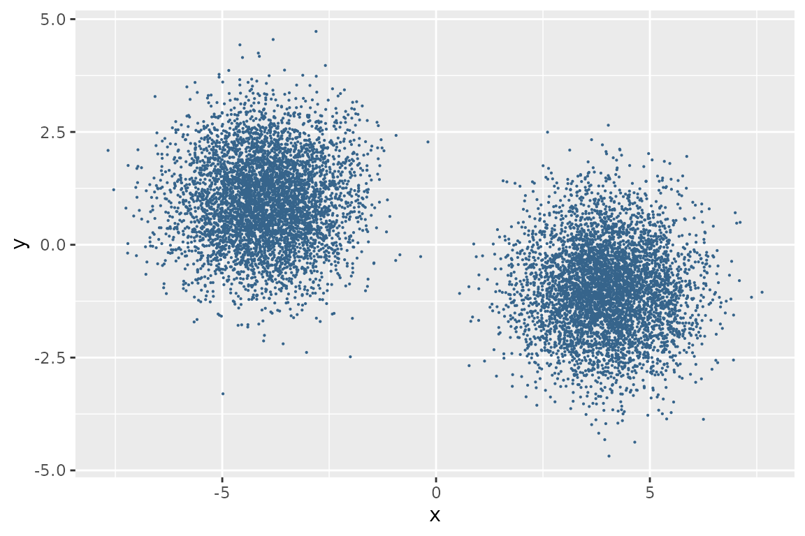

Make 1D grid

Then a one-dimensional grid is built. A one-dimensional grid is defined by the lower bound, the upper bound, and the number of vertical stripes.

# check the extreme values of the points along x
min(df_points$x)
#> [1] -7.6713
max(df_points$x)
#> [1] 7.624361
 
# define boundaries of grid
(xmin <- floor(min(df_points$x)))
#> [1] -8
(xmax <- ceiling(max(df_points$x)))
#> [1] 8
   
# define the grid
grid1d <- makeGrid1d(xmin = xmin, xmax = xmax, xcell = 16)
grid1d
#> class        : Grid1d
#> dimensions   : xcell = 16
#> range        : xmin = -8, xmax = 8

The criterion for defining the grid boundaries and the number of strips varies from time to time based on the data and the type of analysis.

Get the boxplot

Finally we get the boxplot using getBoxplot() function. The getBoxplot() function takes as input an object of class Grid1d and a dataframe of points. If the input dataframe has more than two columns, the first two will be automatically selected.

df_boxplot <- getBoxplot(grid1d, df_points)
    
head(df_boxplot)
#>    xbp         x           y
#> 1 -4.5 -4.626454  0.19566840
#> 2 -3.5 -3.816357 -0.05652565
#> 3 -4.5 -4.835629 -0.03539578
#> 4 -2.5 -2.404719 -0.18556035
#> 5 -3.5 -3.670492  0.49956049
#> 6 -4.5 -4.820468  0.47501129

getBoxplot() assigns the same x value to all points within the same strip. The xbp column is a factor.

ggplot(df_boxplot)+
  geom_boxplot(aes(x = xbp, y = y), fill = "steelblue3", color = "grey40") + 
  labs(x = "x") + 
  scale_x_discrete(breaks = levels(df_boxplot$xbp), drop = FALSE)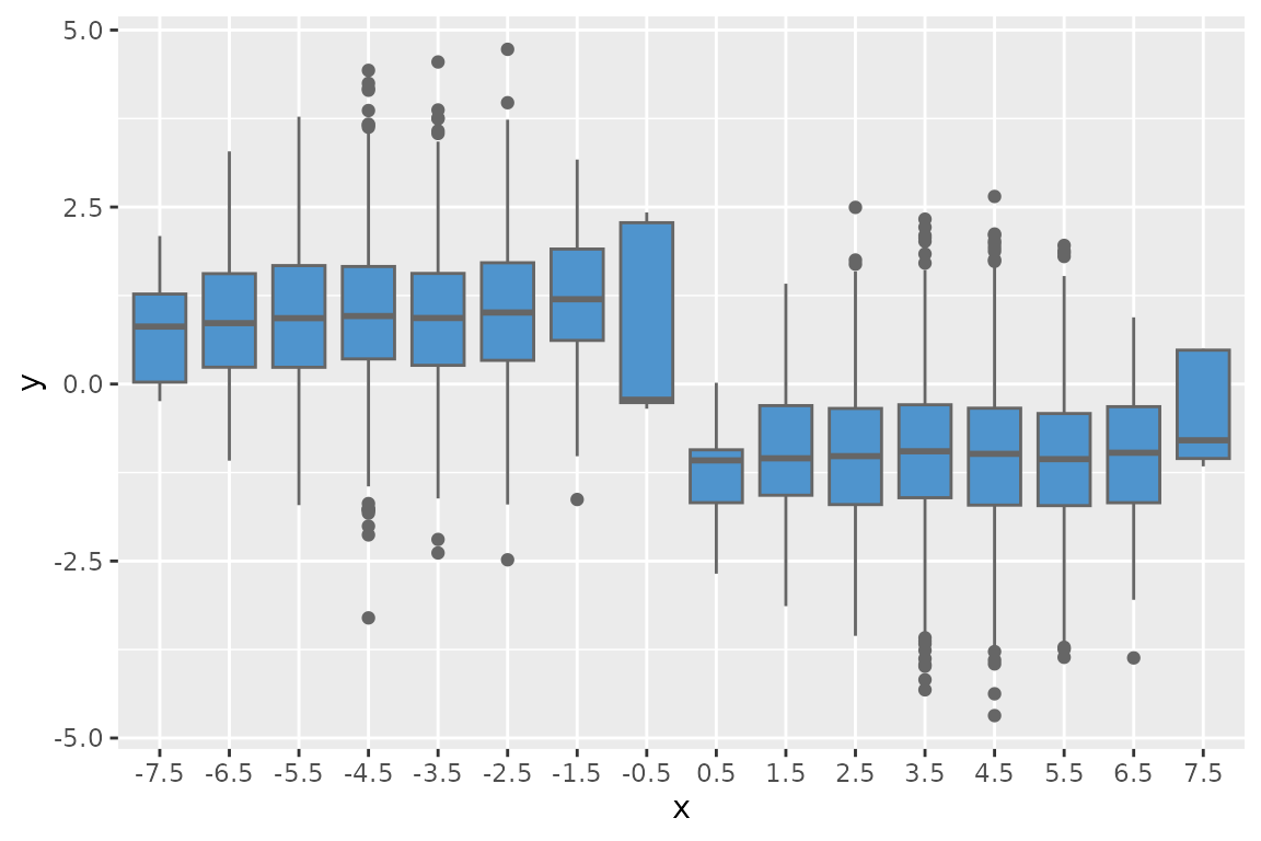

Histogram

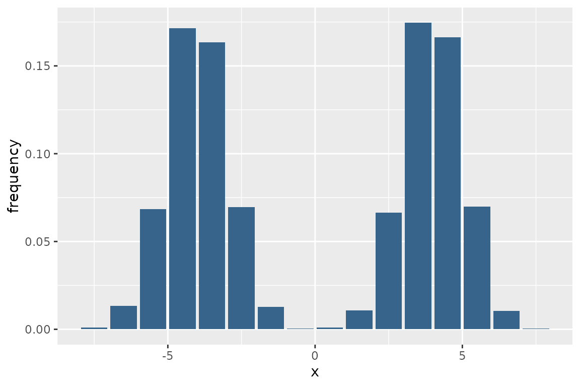
There are functions that can generate a histogram and provide all the information about it. However, a histogram can also be obtained using the getCell() and getCounts() function of rgrids.

getCell() function assigns each point of the plane to its respective strip, counting strips from left to right, while getCounts() function counts how many points fall within each strip and returns a dataframe with two columns: the center of the bin (i.e. the center of the strip) and the count.

df_points$grid_index <- getCell(grid1d, df_points)
#> Warning in getCell(grid1d, df_points): data.frame passed to a Grid1d object;
#> only first column was selected
head(df_points)
#>           x           y grid_index
#> 1 -4.626454  0.19566840          4
#> 2 -3.816357 -0.05652565          5
#> 3 -4.835629 -0.03539578          4
#> 4 -2.404719 -0.18556035          6
#> 5 -3.670492  0.49956049          5
#> 6 -4.820468  0.47501129          4

df_hist <- getCounts(grid1d, df_points$grid_index)
head(df_hist)
#>      x counts
#> 1 -7.5      9
#> 2 -6.5    132
#> 3 -5.5    683
#> 4 -4.5   1715
#> 5 -3.5   1634
#> 6 -2.5    695

ggplot(df_hist) + 
  geom_col(aes(x, counts/sum(counts)), fill = "steelblue4") + 
  labs(y = "frequency")