2D grids

This vignette shows how to perform a density analysis on a plane.

This is only one of the possible analyzes that can be carried out by dividing the plane into a grid.

library(rgrids)
library(ggplot2)

Doing a density analysis can be annoying in some circumstances. To assign points to each element of the grid in the worst case scenario, a double for loop is performed on rows and columns. Let’s see how to make the process painless.

Define dataframe of points

First, a set of random points is generated

set.seed(1)

df_points <- data.frame(x = c(rnorm(n = 50000, mean = -2), 
                              rnorm(n = 50000, mean = 2)), 
                        y = c(rnorm(n = 50000, mean = 1), 
                              rnorm(n = 50000, mean = -1))
) 

head(df_points)
#>            x         y
#> 1 -2.6264538 1.7914415
#> 2 -1.8163567 1.3921679
#> 3 -2.8356286 0.5273330
#> 4 -0.4047192 0.5420483
#> 5 -1.6704922 0.8318681
#> 6 -2.8204684 1.5856737

ggplot(df_points) + 
  geom_point(aes(x, y), color = "steelblue4", size = 0.1)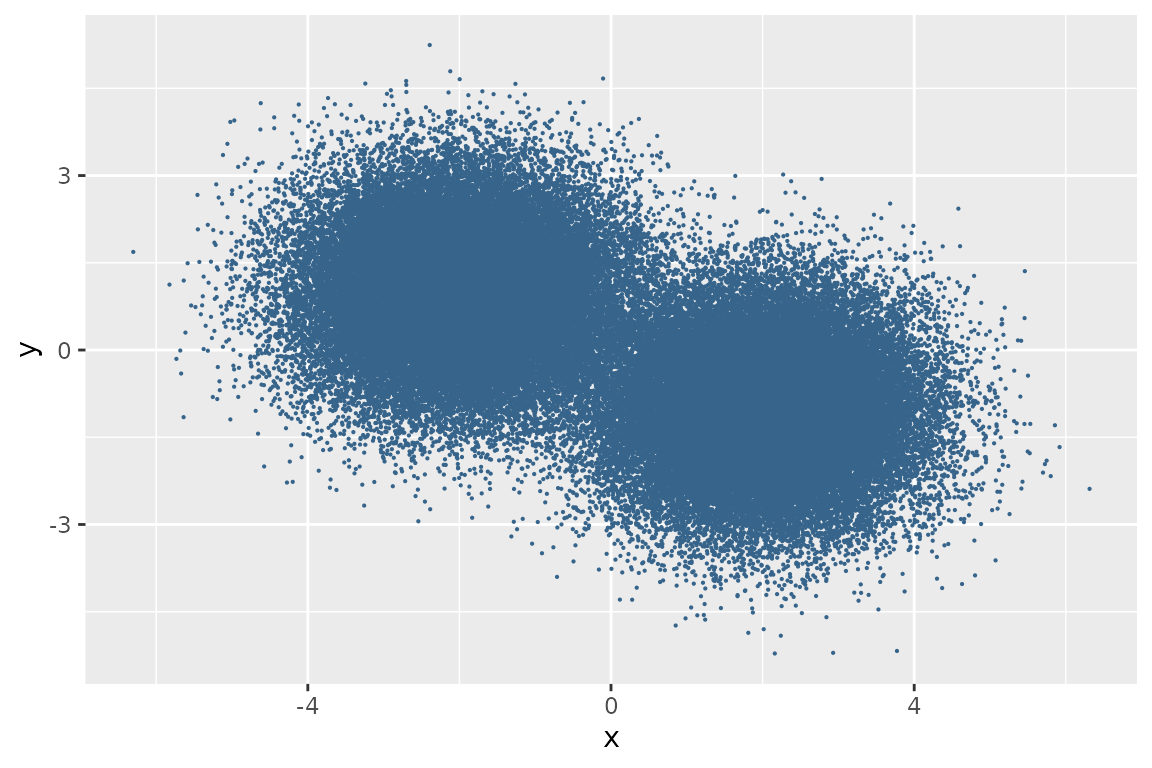

Make 2D grid

Then a two-dimensional grid is built. A two-dimensional grid is defined by lower and upper bound along $x$ and $y$, and the number of cell along $x$ and $y$.

# check the extreme values of the points along x
min(df_points$x)
#> [1] -6.302781
max(df_points$x)
#> [1] 6.313621

# check the extreme values of the points along y
min(df_points$y)
#> [1] -5.218131
max(df_points$y)
#> [1] 5.244194

# define boundaries of grid
(xmin <- floor(min(df_points$x)))
#> [1] -7
(xmax <- ceiling(max(df_points$x)))
#> [1] 7
(ymin <- floor(min(df_points$y)))
#> [1] -6
(ymax <- ceiling(max(df_points$y)))
#> [1] 6

# define the grid
grid2d <- makeGrid2d(
            xmin = xmin, xmax = xmax, xcell = 50,
            ymin = ymin, ymax = ymax, ycell = 50
          )
grid2d
#> class      : Grid2d
#> dimensions : xcell = 50, ycell = 50, ncell = 2500
#> range      : xmin = -7, xmax = 7
#>              ymin = -6, ymax = 6
#> by         : h, count starts from xmin, ymin (bottom-left) 
#>              and x increase faster

In addition to the extremes and the number of cells, makeGrid2d() takes as input an additional parameter by which numbers the elements of the grid by increasing the $x$ (h) or the $y$ (v) faster:

by = "h"      by = "v"
7 8 9         3 6 9
4 5 6         2 5 8
1 2 3         1 4 7

In both cases the count starts from bottom left.

Assign points to cells

Each point of the dataframe is assigned to its respective grid cell via getCell(). The getCell() function takes as input an object of Grid2d class and a matrix or dataframe of points; if the passed matrix or dataframe has more than two columns, the first two will be automatically selected.

grid_index <- getCell(grid2d, df_points)
df_points$grid_index <- grid_index

head(df_points)
#>            x         y grid_index
#> 1 -2.6264538 1.7914415       1616
#> 2 -1.8163567 1.3921679       1519
#> 3 -2.8356286 0.5273330       1365
#> 4 -0.4047192 0.5420483       1374
#> 5 -1.6704922 0.8318681       1420
#> 6 -2.8204684 1.5856737       1565

The values of grid_index column range from 1 to 2500, which is the number of elements in the grid.

Count the points

To get the occurrence of points in each cell just manipulate the previous result and get the grid coordinates. To facilitate the operation, use getCounts() function that takes grid2d and grid_index as input and returns a dataframe of three columns: the first two represent the coordinates of each element of the grid and the third represents the occurrence of points in each cell

df_grid <- getCounts(grid2d, grid_index)

head(df_grid)
#>       x     y counts
#> 1 -6.86 -5.88      0
#> 2 -6.58 -5.88      0
#> 3 -6.30 -5.88      0
#> 4 -6.02 -5.88      0
#> 5 -5.74 -5.88      0
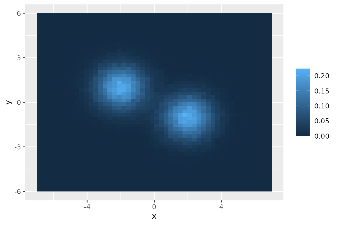
#> 6 -5.46 -5.88      0

Finally, the grid is represented

ggplot(df_grid) + 
  geom_raster(aes(x, y, fill = counts/nrow(df_grid))) + 
  theme(legend.title = element_blank())